Miguel’s muon detector physics paper (website version)

Author: Miguel Ríos Martín

The following article discusses the physics underpinning the Cosmic Watch Muon Detectors and explains how the data displayed on the graphs in the LRO Grafana dashboard (https://cosmicwatch.astronomy.me.uk) are calculated, with detailed explanations of those graphs.

From Axani’s article

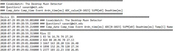
From the article published by Axani et al. about the detector:

• S. N. Axani, J. M. Conrad, & C. Kirby, “The Desktop Muon Detector: A simple, physics-motivated machine- and electronics-shop project for university students”, American Journal of Physics, 85(12), 948–958 (2017).

Key summary data:

• 80–90% of muons reaching Earth’s surface have energies in the GeV–TeV range.
• Average muon energy at sea level: 4 GeV.
• Energy loss in the ionization region (via electromagnetic interactions) is nearly constant, averaging 2.2 MeV/cm.
• Data from two detectors operating in coincidence mode correspond to muon detections.
• Muon flux with E > 1 GeV at sea level (horizontal detector): 1 cm⁻² min⁻¹, accounting for the full celestial hemisphere (2π sr).
• Detector output via USB includes: [data specifics from the original article, if any].

Flow estimates

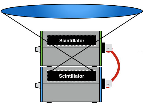
For two detectors in coincidence mode, positioned horizontally and one above the other:  

We have:

• The surface area of the scintillator is 25 cm² (5 cm × 5 cm).
• We assume the scintillators are separated by 3 cm.
• The solid angle subtended by two 5 cm × 5 cm plates separated by 3 cm is 3.3 sr.(Reference: R. J. Mathar, “Solid angle of a rectangular plate”, Max-Planck Institute of Astronomy, 1–9 (2015).)
• The solid angle subtended by the complete celestial vault is 2π sr.
• The theoretical flux (F_teor) for the entire celestial vault is 1 cm⁻² min⁻¹.

If we call (F_exp) the flux detected by the detectors, we have (in counts per second, cps): 

F_exp = F_teo x (scintillator surface) x (solid angle of two sheets) / (solid angle of complete vault x 60 seconds)

In this case it should be 

F_exp = 1 x 25 cm^2 x 3,3 sr /(2 Pi x 60 seconds) = 0.219 cps

(This is an approximation because the flux is not uniform in all directions.) 

Explanation of some graphics 

• Graph 1: “Muon flux in cm⁻² min⁻¹ – Normalized (celestial vault)”. We have calculated F_teor from the F_exp measured by each detector, in units of cm⁻² min⁻¹. 
• Graph 2: The muon flux is calculated over the past 24 hours in 5-minute intervals, and the current percentage change is determined as: 

F(24 hours) -> The flux over the past 24 hours, in 5-minute intervals. 

F(now) -> The current flux over the last 5 minutes. 

% = (F(now) – F(24 hours)) / F(24 hours) x 100 

This gives an estimate of the increase or decrease in muon flux relative to the past 24 hours. 

• Graph 3: The variation is calculated over an interval (f_0) of N muons (buffer size = N). This is: 

f_0 -> Arrival frequency of N muons: N/t_r(N muons). 

where t_r(N) is the actual arrival time of N muons (discounting detector dead time). 

mean(f_0) -> This is the average value of f_0 over the time window specified by the graph. 

We calculate: 

% = (f_0 – mean(f_0))/mean(f_0) x 100 

This gives an estimate of the flux variation, in percentage, for every 150/600 muons detected. 

With flux-change-OULU:

We measure the percentage change in the neutron flux (nmdb) arriving at Earth at the Oulu Observatory (Finland) within the time window selected in the graph. 

In theory,
The variations recorded in cosmic rays detected at Earth’s surface should also be reflected in the muon flux, since cosmic rays are the source of muons.

Muon frequency (Burst)

The muon flux is not uniform over time, as is evident from the appearance of bursts.

The method I used for burst detection was as follows:

• We select the size of the buffer N (buffer size = N).
• We record the detection times of N muons (real times, excluding detector dead times): {t1, t2, …,tN}.
• For each time ti, the frequency of order j is calculated, with j = 1, 2, 3, 4, 5. This is done by considering the time of the j muons before and the j
• muons after muon i, that is:

f_j (i) = (2j + 1)/(t_(i+j) – t_(i-j))

f_j (i) represents the arrival frequency of (2j + 1) muons at time t_i. Half of the muons arriving before and half after are counted. This is done for groups of 3, 5, 7, 9, 11 muons at each time.

f_0(i) = N/t(N muons).

f_0(i) is a reference as it uses a buffer of N muons.

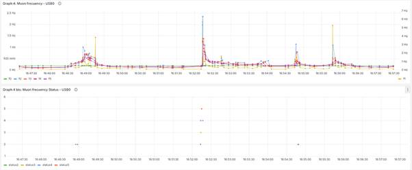
• Graph 4: Shows the different frequencies on the detector connected to the USB0 port.
• Graph 5: Shows the different frequencies on the detector connected to the USB1 port.

By comparing f_0(i) with f_j (i) we can estimate the characteristics of the bursts received by the detector. 

If f_1 is much larger than f_0, we will have received 3 muons in a short period of time. 

If f_5 is much larger than f_0, we will have received 11 muons in a short period of time.

• An anomaly has been considered when the partial frequency exceeds the buffer frequency by a factor of ‘anomaly_threshold‘:

Anomaly at level j and time i ⇒ fj(i) > (anomaly_threshold) f0(i).

• An anomaly at f1 means that a 3-muon burst has been detected, which we can consider a short burst.
• On the other hand, an anomaly at f5 represents an 11-muon burst.
• When all partial frequencies show anomalies, we have what we call a sustained burst. Eleven muons are received over a period of time, so all partial frequencies are elevated (anomalous)compared to the average buffer frequency.

To measure the inhomogeneity of the muon arrival rate, several levels are established using status. When two anomalies occur, that is, two values of j for which an anomaly occurs, we set status = 2. With 3 anomalies, status = 3.

When all frequencies represent an anomaly, we say that status = 5, that is, f_j > (anomaly-threshold) f_0, for all values of j: 1, .., 5.

The value of status = 5 establishes the instants where the bursts are most pronounced in terms of the number of muons and time.

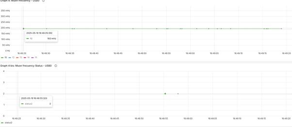
Graph 4 bis: Allows us to observe when and what type of bursts occur at USB0.

Graph 5 bis: Allows us to observe when and what type of bursts occur at USB1.

The following numerical graphs show the maximum, average, and minimum frequencies for each detector on the USB0/1 channels.

For example, we can see that the minimum detected period for 3 muons to arrive is:

T(3 muons)_min = 1/f_1(max) = 1/214 = 0.47 ms

and the maximum period without detecting 3 muons is:

T(3 muons)_max = 1/f_1(min) = 1/0.0336 = 29.8 s

The minimum time for 11 muons to be received is:

T(11 muons)_min = 1/f_5(max) = 0.6 s

Grafana’s structure and graphics allow for zooming in to gain more detail about the bursts. For example, on 19-0-2025 at 16:48:25, 20 muons were received in a space of 1 second:

Other observations can be made with the possibilities offered by Grafana that show the shape of the bursts: 

Graph 6: “Allows you to detect the moments when the highest frequencies occur in each detector by selecting the channel, frequency, and its maximum value from the menus above. The graph changes as you select different options from the menus. 

Muon coincidence

According to the CosmicWatch muon detector documentation, the uncertainty in the times measured by the Arduino is 1 ms. Since the value of t_r comes from a difference in times, we can consider that its uncertainty is 2 ms. Remember that: 

• t_a -> Time measured by the Arduino from the start 
• t_d -> Arduino dead time (not operational) 
• t_r = t_a – t_d

Reviewing the recorded numerical data, it is found that occasionally two events have the same t_r even though their t_a values are different. The equality of t_r  can be an indicator that both events occurred at the same time, even though they have different t_a values (and obviously also different t_d values). The figure shows the explanation: 

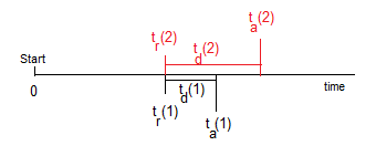
Given two events (1) and (2), they will be coincident if their real time difference (t_r) is zero, plus or minus the uncertainty of the sum of both. This means that they can coincide if

|t_r(2) – t_r(1)| <= 4 ms

In Graph 6 bis, this difference can be observed for each of the channels (USB0/1) and the time instant at which they occur. 

SIPM

Another interesting aspect to analyse is the value provided by the photomultiplier (SiPM).

From Axani’s article, we deduce that if the average energy with which muons reach Earth is approximately constant, then the size of the SiPM must be related to the distance the muon travels in the scintillator.

Graph 7: This shows the histogram of the SiPM values detected in both detectors, using a 1 mV scale. It is interesting to note that the most frequently occurring value in both detectors is between 80 and 81 mV (note that the average for both is 80.1 mV). If we infer that the most commonly travelled distance by the muon is 1 cm (the thickness of the scintillator is 1 cm), then we can assume that 80.1 mV corresponds to a travel distance of 1 cm, which is what has been used to produce Graph 8, converted into centimetres travelled.

The second maximum, for both detectors, also clearly coincides at 97–98 mV.

Also surprising is the relative maximum that appears, for both detectors, around 22 mV. So far, I do not have a clear explanation for this.

Graphs 9 and 10: These represent the normalized histogram of SiPM values for USB0/1. That is, the different SiPM values scaled in 1 mV intervals (horizontal axis) versus the normalized frequency of occurrence (vertical axis). The sum of all frequencies is 1.