For 1420 MHz (the H I line at 1420.4058 MHz), the “best” cavity filter depends on where you place it in the chain (pre-LNA vs post-LNA) and what you need to reject. Below are practical, astronomy-focused specs that work very well in the field.

Recommended target specs (bandpass cavity filter, 50 Ω)

• Center frequency (f₀): 1420.406 MHz (tunable ±2–3 MHz via screws)
• Passband bandwidth (-3 dB):
  • 10 MHz (good all-round preselector for spectral work)
  • 20 MHz (if you want looser passband and lower insertion loss)
  • Rationale: even ±300 km/s Doppler shift is only ≈±1.42 MHz, so 10 MHz comfortably covers Galactic velocities while giving good nearby-band rejection.
• Topology / poles: 3- to 4-pole Chebyshev (0.1 dB ripple) or quasi-elliptic (if you want steeper skirts).
  • 3-pole is a great low-loss pre-LNA option; 4-pole buys you much better skirts if you have tough RFI.
• Insertion loss:
  • ≤ 0.5–0.8 dB (3-pole), ≤ 1.0 dB (4-pole) at f₀ (critical if used pre-LNA).
• Return loss: ≥ 15 dB across passband (≥ 20 dB ideal).
• Out-of-band rejection (typical goals):
  • ≥ 40 dB at ±25 MHz from f₀
  • ≥ 60 dB at ±40 MHz (helps with services near 1.45 GHz)
  • ≥ 80 dB by ±100 MHz (keeps strong out-of-band energy out of the front-end/LNA).
• Group delay variation (over passband): ≤ 150 ns (10 MHz BW) to preserve spectral line shape.
• Power handling: Not critical for RX; ≥ +20 dBm is ample.
• Temperature stability: Drift ≤ ±5 ppm/°C (aim for silver-plated copper cavities, low-TCR hardware); include lock nuts after tuning.
• Connectors: N-type female (50 Ω) or SMA if fully lab-grade and mechanically protected.
• Mechanical: Air-dielectric coaxial cavities (silver-plated copper or brass), unloaded Q ≈ 3000–8000. Use rigid coupling loops/pins with adjustable iris/screws for inter-resonator coupling.
• Shielding: Seam-welded or well-gasketed enclosure; internal partitions between resonators to minimize parasitics.

---

Two proven “good” configurations

A) Pre-LNA preselector (minimal noise hit)

• Use case: Right after the antenna, before the first LNA.
• Spec: 3-pole Chebyshev, 10 MHz BW, IL ≤ 0.6 dB, RL ≥ 18 dB, rejection ≥ 55 dB @ ±40 MHz.
• Why: Keeps strong off-band energy out of the LNA while adding very little to the system noise temperature.

B) Post-LNA cleanup (tough RFI)

• Use case: Immediately after a low-NF LNA.
• Spec: 4-pole quasi-elliptic, 10–15 MHz BW, IL ≤ 1 dB, RL ≥ 18 dB, deep skirts (≥ 70 dB by ±40–50 MHz).
• Why: With SNR already boosted by the LNA, you can afford a bit more loss to get aggressive rejection of nearby services (e.g., around 1450 MHz).

---

Practical notes for 1420 MHz astronomy

• Bandwidth choice:
  • 10 MHz passband is a sweet spot: wide enough for all Galactic H I velocities and Earth/Sun motions, yet narrow enough to meaningfully preselect.
  • If you only do continuum imaging or need maximum sensitivity pre-LNA, a 20 MHz passband can shave ~0.2–0.3 dB insertion loss.
• Order (poles):
  • 3-pole for low IL before LNA.
  • 4-pole when RFI is nasty or when placed after LNA.
• Materials & finish: Silver-plate the resonator rods and cavity walls; use clean, tight RF gaskets; avoid ferrous hardware inside the RF volume.
• Tuning workflow:

• Individually peak each cavity at 1420.406 MHz (weak coupling).
• Set inter-cavity coupling to hit the target BW.
• Iterate source/load coupling for RL and IL.
• Finalize with warm-up to operating temperature and re-touch.
• System placement tips:
  • If very strong out-of-band signals are present, put a low-loss 3-pole cavity before the LNA.
  • Add a sharper 4-pole after the LNA (or before the SDR) to protect the ADC and clean the band further.

---

Example spec sheet you can hand to a fabricator

• Type: Coaxial cavity bandpass filter, 50 Ω
• Center: 1420.406 MHz (mechanically tunable ±3 MHz)
• Order: 3-pole Chebyshev (0.1 dB ripple)
• BW (-3 dB): 10.0 ± 0.5 MHz
• Insertion Loss: ≤ 0.6 dB @ f₀; ≤ 0.9 dB over passband
• Return Loss: ≥ 18 dB over passband
• Rejection: ≥ 55 dB at 1380 MHz and 1460 MHz; ≥ 75 dB at ≤ 1320 MHz and ≥ 1520 MHz
• Group Delay Ripple: ≤ 120 ns pk-pk over passband
• Power: ≥ +20 dBm CW (receive-only)
• Temperature: Drift ≤ ±5 ppm/°C; locking hardware provided
• Connectors: N-female both ends (SMA optional)
• Finish: Silver-plated internal RF surfaces; black anodized exterior
• Size: Typical for 3-resonator 1.4 GHz unit (fabricator to optimize for Q and IL).

External-Q Targets and VNA Tuning Plan:

Here are coupling/external-Q targets and a tight VNA tuning plan for a 3-pole, 0.1 dB-ripple Chebyshev cavity bandpass at the H I line.

Equations in following are more visible in attached.

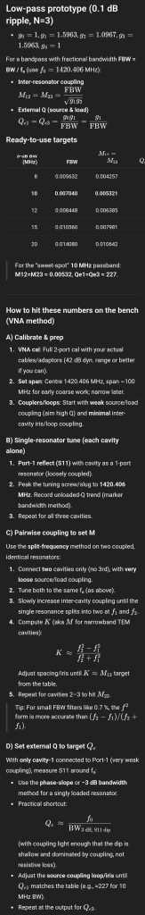
Low-pass prototype (0.1 dB ripple, N=3)

• (g_0=1), (g_1=1.5963), (g_2=1.0967), (g_3=1.5963), (g_4=1)

For a bandpass with fractional bandwidth FBW = BW / f₀ (use (f₀=1420.406) MHz):

• Inter-resonator coupling
  ( M_{12}=M_{23}=\dfrac{\text{FBW}}{\sqrt{g_1 g_2}} )
• External Q (source & load)
  ( Q_{e1}=Q_{e3}=\dfrac{g_0 g_1}{\text{FBW}}=\dfrac{g_1}{\text{FBW}} )

Ready-to-use targets

3-dB BW (MHz)	FBW	(M_{12}=M_{23})	(Q_{e1}=Q_{e3})
8	0.005632	0.004257	283.42
10	0.007040	0.005321	226.74
12	0.008448	0.006385	188.95
15	0.010560	0.007981	151.16
20	0.014080	0.010642	113.37

For the “sweet-spot” 10 MHz passband: M12=M23 ≈ 0.00532, Qe1=Qe3 ≈ 227.

---

How to hit these numbers on the bench (VNA method)

A) Calibrate & prep

1. VNA cal: Full 2-port cal with your actual cables/adaptors (42 dB dyn. range or better if you can).
2. Set span: Centre 1420.406 MHz, span ~100 MHz for early coarse work; narrow later.
3. Couplers/loops: Start with weak source/load coupling (aim high Q) and minimal inter-cavity iris/loop coupling.

B) Single-resonator tune (each cavity alone)

1. Port-1 reflect (S11) with cavity as a 1-port resonator (loosely coupled).
2. Peak the tuning screw/slug to 1420.406 MHz. Record unloaded-Q trend (marker bandwidth method).
3. Repeat for all three cavities.

C) Pairwise coupling to set M

Use the split-frequency method on two coupled, identical resonators:

1. Connect two cavities only (no 3rd), with very loose source/load coupling.
2. Tune both to the same f₀ (as above).
3. Slowly increase inter-cavity coupling until the single resonance splits into two at (f_1) and (f_2).
4. Compute ( K ) (aka (M) for narrowband TEM cavities):
   [
   K ;\approx; \frac{f_2^2 – f_1^2}{f_2^2 + f_1^2}
   ]
   Adjust spacing/iris until (K \approx M_{12}) target from the table.
5. Repeat for cavities 2–3 to hit (M_{23}).

Tip: For small FBW filters like 0.7 %, the (f^2) form is more accurate than ((f_2 – f_1)/(f_2 + f_1)).

D) Set external Q to target (Q_e)

With only cavity-1 connected to Port-1 (very weak coupling), measure S11 around f₀:

• Use the phase-slope or −3 dB bandwidth method for a singly loaded resonator.
• Practical shortcut:
  [
  Q_e ;\approx; \frac{f_0}{\text{BW}_{\text{3 dB,,S11 dip}}}
  ]
  (with coupling light enough that the dip is shallow and dominated by coupling, not resistive loss).
• Adjust the source coupling loop/iris until (Q_{e1}) matches the table (e.g., ≈227 for 10 MHz BW).
• Repeat at the output for (Q_{e3}).

E) Assemble all 3, final tune on S-parameters

1. Cascade all three. Start with the previously set M’s and Qe’s.
2. Observe S21: You should see ~Chebyshev ripple (≈0.1 dB) across the passband and the correct −3 dB bandwidth.
3. Iterate very small tweaks:
   • Inter-cavity coupling sets total BW and skirt steepness.
   • Source/load coupling trades passband ripple vs return loss.
   • Re-touch each resonator screw to keep centre at 1420.406 MHz after mechanical changes.
4. Targets to confirm:
   • IL ≤ 0.6–0.8 dB (3-pole)
   • RL ≥ 18–20 dB across passband
   • BW within ±0.5 MHz of goal
   • Ripple ~0.1 dB (Chebyshev signature)
   • Skirts meet your earlier rejection goals (e.g., ≥55 dB @ ±40 MHz for the pre-LNA unit).

---

Turning M and Qe into physical settings

• Inter-resonator M grows with larger iris aperture, closer loop spacing, or stronger probe alignment; reduce M by increasing gap or rotating loops to reduce mutual coupling.
• External Qe increases (weaker coupling) as you pull the input/output loop away from the E-field region, shrink loop area, or rotate it to reduce magnetic coupling.
• Make adjustments symmetrically to keep passband flatness; if ripple is higher near one edge, that side’s Qe/M is slightly off.

---

Quick sanity checks

• If passband is too narrow: (M)s are too small or (Q_e)s too high (too weak).
• If passband is too wide: (M)s are too large or (Q_e)s too low (over-coupled).
• If deep notch in passband: one resonator off-frequency; re-peak each cavity with the others temporarily de-coupled.

---