Meteors vary enormously in size, depending on the original meteoroid (the solid body before it enters Earth’s atmosphere). Here’s a breakdown by category:
| Type | Typical Size (Diameter) | Description |
| Micrometeoroids | < 1 mm | Dust-sized particles, often from comets; produce faint streaks or are invisible. |
| Small Meteoroids | 1 mm – 1 cm | Common “shooting stars” seen during meteor showers. These completely burn up in the atmosphere. |
| Medium Meteoroids | 1 cm – 10 cm | Produce very bright meteors or fireballs; some fragments may survive as meteorites. |
| Large Meteoroids | 10 cm – 1 m | Very bright bolides; can produce sonic booms and ground impacts. |
| Asteroidal Meteoroids / Small Asteroids | 1 m – 10 m | Rare; atmospheric entry releases energy comparable to small nuclear blasts (e.g. Chelyabinsk, 2013). |
| Asteroids | > 10 m | Too large to be called meteoroids; most would produce catastrophic impacts if they hit Earth. |
Summary of Meteor Terminology
- Meteoroid – object in space, typically mm–m in size.
- Meteor – the luminous streak seen as it burns in the atmosphere.
- Meteorite – any fragment that survives to reach the ground.
Excellent question — and a key one in meteor science.
The size (or mass) frequency distribution of meteoroids follows a very steep power law, meaning small ones are vastly more common than large ones.
🔹 General Form of the Distribution
The differential mass distribution is usually expressed as:
[
N(m),dm = k,m^{-s},dm
]
where:
- (N(m),dm) = number of meteoroids with masses between (m) and (m + dm)
- (k) = normalization constant
- (s) = mass index, typically 1.6–2.2 for meteoroids
Equivalently, in terms of diameter (D) (assuming constant density):
[
N(D) \propto D^{-q}
]
where (q = 3s – 2).
Typical (q) values ≈ 2.5–3.5.
🔹 Interpretation
| Mass (grams) | Approx. Diameter | Relative Frequency | Typical Phenomenon |
| (10^{-6}) g | 0.1 mm | Extremely common | Micrometeors, zodiacal dust |
| (10^{-3}) g | 1 mm | Common | Normal meteors during showers |
| (1) g | 1 cm | ~1 in 10⁶ compared to mm-size | Bright meteor |
| (10^3) g | 10 cm | ~1 in 10⁹ | Fireball, potential meteorite |
| (10^6) g | 1 m | ~1 in 10¹² | Bolide, impactor (rare) |
Roughly speaking, for every factor of 10 increase in size, the number drops by about 100–1000×.
🔹 Observational Evidence
- Radar and optical surveys (e.g. CMOR, AMOR, and NASA’s photographic networks) confirm (s ≈ 1.8) for most sporadic and shower meteoroids.
- Spaceborne micrometeoroid detectors (e.g. LDEF, Pegasus, etc.) show the same law down to micron sizes.
- The distribution steepens at smaller sizes (<0.1 mm) because of Poynting–Robertson drag and solar radiation pressure removing dust more efficiently.
🔹 Visualization (in words)
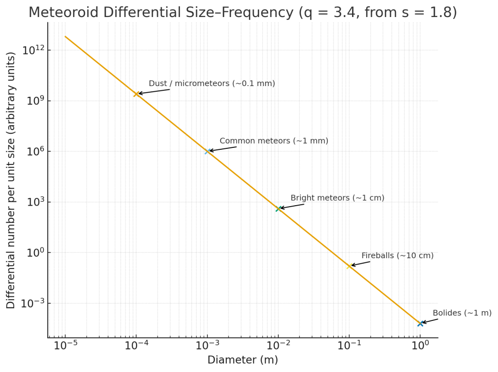
If you plotted log(number) vs log(size), you’d see a nearly straight line sloping downward — very steep — indicating an inverse power relationship:
lots of dust, few big rocks.
Would you like me to generate a graph (log–log plot) showing this size–frequency relationship with real parameter values (e.g., (s = 1.8)) and annotated meteor categories?
Here’s a log–log plot of the differential size–frequency (n(D)\propto D^{-q}) using a typical meteoroid mass index (s=1.8) → size index (q = 3s-2 = 3.4). I’ve annotated common categories (dust → bolides).